Terminology – ostrogothia

Nomina si nescis, perit et cognitio rerum.
(If you know not the names of things, the knowledge of things themselves perishes.)
Carl von Linné

Active inference framework

System: An arrangement of interacting elements that together realize functions. Examples include information systems, biological organisms, ant hills, medical devices, and space stations. In the context of active inference, system often refers to the body or the environment of an organism. A system can also refer to a lower-level controller in a hiearchy of controllers. A controller controlled by a controller.

Open system: A system that has external interactions. Such interactions can take the form of information, energy, or material transfers into or out of the system boundary.

Non-equilibrium steady state (NESS): A stable, physical state of an open system that is constantly kept out of equilibrium by external forces, such as energy, matter, or information flux. Unlike equilibrium, NESS features persistent currents (e.g., heat flow, particle transport), continuous entropy production, and is maintained through constant interaction with its environment. Living organisms are in a NESS.

Predictive control: An advanced control strategy that uses a dynamic system model to predict future behavior over a time horizon.

Active inference: A general form of predictive control consisting of planning an generation of action states to control an allostatic system to keep it on a viable manifold by minimizing a quantity called free energy. All control algorithms capable of sustaining NESS are subsets of active inference.

Allostatic system: An open system with an internal controller that generates its own counter-gradients (via effectors) to modulate its boundary conditions, ensuring its continued existence in a NESS regardless of external environmental fluctuations. Examples are to varying degrees a liver cell, a human, a tribe, a society, and planet Earth.

Controller: A stateful system that gets information about the state of a controlled system via transducers and controls it via effectors so as to keep the controlled system on its viable manifold (in a NESS). Active inference posits a hierarchy of controllers. The lowest-level controller regulates the physical states ($\eta$) of the controlled system. Higher-level controllers regulate the information state of the controller beneath it in the hierarchy. For the higher-level controller, the next lower-level controller is its controlled system.

The physical realization of a controller is often part of the system it controls. The human brain is, for instance, a part of the human body.

When the controlled system is a lower-level controller, the interactions occurs entirely within the information domain. In these higher-level architectures, “transducers” and “effectors” are not physical organs (like biological eyes or limbs). Instead, they are informational interfaces – the specific computational mappings and synaptic projections that form the Markov blanket between the hierarchical layers. They filter lower level states into higher-level observations, and translate higher-level actions into lower-level empirical setpoint distributions.

Generative process: The dynamics of an open system.

Physical state, $\eta$: The thermodynamic, chemical, or mechanical arrangement of a system’s matter and energy. The physical viable manifold ($\mathcal{M}_\eta$) is defined in terms of physical states; if an allostatic system’s physical state drifts off its viable manifold, it loses its non-equilibrium steady state (NESS) and ceases to exist.

The physical state evolves according to the equation:

$$d\eta = f(\eta)dt + d\omega_\eta$$

where $\omega_\eta$ represents random perturbations of the state.

Examples: The physical temperature of the human body, the ATP concentration in a cell, the momentum of a vehicle.

Information state, $s, o, a$: A random variable representing a quantity of interest such as a controller state.

An information state supervenes on a physical substrate like the brain or a computer memory.

Examples: Observation, action, object category, color, generalized coordinates of motion (position, speed, acceleration,…).

Controller state, $s$: An information state within the controller. The three types of controller information states are:

Observation, $o$: Represents the observable state of the controlled system as transformed by a sensor.
Action, $a$: Generated by the controller to induce an action state in the controlled system through an effector.
Representational state, $s$: Represents the state of the controlled system, excluding the observation or the action.

Representational state, $s$: A specific type of information state within a controller that represents the state of the controlled system. Unlike an observation ($o$), which is a direct transformation of an observable state ($\eta_o$), a representational state is an inferential construct that “stands in for” the physical state ($\eta$) within the generative model.

The representational state is the random variable over which the recognition distribution $q(s \mid \theta)$ is defined.

Because generative models are typically hierarchical, representational states vary in their level of abstraction. Low-level representational states represent immediate, localized physical states ($\eta$) of the controlled system, e.g., $\text{current joint angle}$. High-level representational states are compressed, complex, long-term configurations of lower-level states such as $\text{social status}$ or $\text{navigational goal}$.

Because $s$ is a representation and not the thing itself, it can be “wrong” (manifesting as prediction error) or “counterfactual” (representing states that are used in planning but not yet realized).

Observable state, $\eta_o, s_o$: The subset of a system state that can be sensed by the controller’s transducers to produce an observation $o$ in the controller.

Within a hierarchy of controllers, the observable state of a controller at level $i$, as observed by the controller at level $i+1$, is the parameter set $\theta$ of its recognition distribution of the level $i$ controller.

Example: The temperature of a system, the mean and the precision of the recognition distribution $q(s \mid \mu, \Pi)$.

Observation, $o$: A controller state representing an observable state as transformed via a transducer.

Action state, $\eta_a$: In case of a physical system, a transient subset of a physical state generated by an effector with the intention to perturb the system’s physical state. The action state is initiated by an action $a$ generated by the controller. The action state works through the system dynamics:

$$d\eta = f(\eta, \eta_a)dt + d\omega_\eta$$

In a hierarchy of controllers, the action state of a controller at level $i$ is a setpoint distribution received from the controller at level $i+1$. It influences the “computational action” of the lower-level controller.

Example: The activation of a muscle triggered by an action in the form of a potential that reaches the end of the motor neuron (the presynaptic terminal). The mean and the precision of the setpoint distribution $p(s \mid \mu, \Pi)$

Action, $a$: A controller state that drives an action state in the controlled system via an effector.

Markov blanket $b$: The set $\eta_b = \{\eta_o, \eta_a\}$ or, if the system is a controller at level $i$ in a hierarchy of controllers, $s_b^{(i)} = \{s_o^{(i)}, s_a^{(i)}\}$. The Markov blanket mediates all information between the controller states and the system states.

Mathematically the Markov property implies that: $p(s, \eta | \eta_b) = p(s | \eta_b)p(\eta | \eta_b)$ or if the Markov blanket separates a controller $\mathcal{C}^{(i+1)}$ and a controlled controller $\mathcal{C}^{(i)}$, $p(s^{(i+1)}, s^{(i)} | s_b^{(i+1)}) = p(s^{(i+1)} | s_b^{(i+1)})p(s^{(i)} | s_b^{(i+1)})$.

The universe consists of many nested systems, each with their own Markov blanket.

Organism: A allostatic system.

Generative model, $p(s, o, a), p(s, o, \pi)$: The controller’s model of the controlled system mathematically relating controller states $s$, observations $o$, and actions $a$ (when describing the reflexive function of the lowest-level controller) or $s$, $o$, and policies $\pi$ (when describing planning).

Structural setpoint distribution, $\tilde p(s), \tilde p(o)$: A hardcoded, phylogenetically endowed, probability distribution over representational states or observations with high probabilities for preferred representational states or observations.

When expressed over observations, it should be understood thus:

$$\tilde p(o) = \int p(o \mid s) \tilde p(s) ds$$

Example: a probability distribution with a sharp peak at the optimal human body temperature of 37°C.

Empirical setpoint distribution, $\tilde p(s), \tilde p(o)$: A probability distribution over representational states or observations dynamically defined by a higher level controller in the controller hierarchy. See also structural setpoint distribution.

Example: a probability distribution with a sharp peak at “hand holding a cup of coffee”.

Setpoint distribution, $\tilde p(s), \tilde p(o)$: A probability distribution over repesentational states or observations that is a combination of a structural setpoint distribution and an empirical setpoint distribution. The setpoint distribution drives the controller to shift the state distribution of the controlled system toward the state distribution represented by the setpoint distribution. See also prior distribution.

Prior distribution, $p(s)$: A probability distribution over controller states that is the controller’s belief about the controller state before an observation has been made; the expected controller state distribution. The prior distribution and the setpoint distribution, when active in a controller, are the same distribution. The term setpoint distribution is used when the main purpose of the distribution is to drive action whereas the term prior distribution is used when the main purpose of the distribution is to guide perception.

Recognition distribution, $q(s \mid \theta)$: The variational distribution that is an approximation of the intractable posterior distribution $p(s \mid o)$. $\theta$ represents the recognition distribution parameters such as the mean and the precision (if a Gaussian).

Generative model parameters, $\phi$: The parameters that define the generative model. Analogous to weights in a deep learning model. Learning leads to a change of $\phi$.

Physical viable manifold, $\mathcal{M}_\eta$: The manifold $\mathcal{M}_\eta$ defined by:

$$\mathcal{M}_\eta = \{ \eta \in \Omega : p(\eta) > \epsilon \}$$

It defines the physical states in which the system is in a non-equilibrium steady state (NESS), i.e., “alive”. As long as a system is in a NESS, then the physical states on the viable manifold are the physical states the system is most likely to be in. Otherwise it wouldn’t be in NESS.

Computational viable manifold, $\mathcal{M}_s$: The bounded set of lower-level information states (acting as higher-level controller’s “physical environment”) within which the controller’s internal model can successfully minimize free energy. If the controlled system’s states drift off this manifold, the controller loses its computational non-equilibrium steady state (NESS) and its algorithm collapses into runaway prediction errors.

Decision, $\pi_t$: A step in a policy (see below) that determines the probabilities for the transitions from representational state $s_t$ to representational state $s_{t+1}$. Mathematically :

$$P(s_{t+1} | s_t, \pi_t) = B_{\pi_t}$$

meaning that

$$q(s_{t+1} \mid \pi_t) = \sum_{s_t} p(s_{t+1} \mid s_t, \pi_t) q(s_t)$$

Where:

$s_{t+1}$ is the representational state at the next time step.
$s_t$ is the current representational state.
$\pi$ is the policy, the hypothetical series of decisions $\pi_t$.
$B$ is the transition matrix representing the state transition probabilities going from time step $t$ to time step $t+1$.

Policy, $\pi$: A series of decisions $\pi_i$ intended to, within the limits of epistemic uncertainty, produce a certain sequence of representational states starting from the current recognition distribution. Epistemic uncertainty means that states need to be represented as probability distributions rather than single values.

Notes

A tilde over a probability distribution, like $\tilde p(s)$ or $\tilde p(o)$, means that the distribution is a setpoint distribution, rather than a neutral predictions about the world.

The table below summarizes the mapping between the terms above and conventional AIF terms.

Term	AIF equivalent	Role
Controller	Agent / brain	The control system controlling the controlled system by minimizing free energy.
System, allostatic system	Generative process	The physical system being controlled.
Physical state	Hidden state	The state of the controlled system.
Controller state, information state	Latent variable	The controller’s “guess” at the system state.
Viable manifold	Attracting set	The “safe” operating envelope of physical states.
Setpoint distribution	Prior	The setpoint for the controller.
Decision	Action	Determines the probabilities for the state transitions in policy inference.

Artificial intelligence

Artificial intelligence (AI): The capability of computational systems to perform tasks typically associated with human intelligence, such as learning, reasoning, problem-solving, perception, and decision-making. “AI” is often used informally as a noun denoting software components with artificial intelligence.

Machine learning: A field of study in artificial intelligence concerned with the development and study of statistical algorithms that can learn from data and generalise to unseen data and thus perform tasks without explicit instructions.

Algorithm: A computational architecture or procedural method that can be trained on data to perform a task. Examples: convolutional neural network, transformer.

Training algorithm: A set of instructions used in machine learning to iteratively adjust the parameters of a model so it can learn from data and make accurate predictions on new data.

Model: A specific, trained AI algorithm. Example: GPT-4o.

Inference engine: A software and/or hardware component that evaluates a trained model on new data and produces output results (e.g., predictions). Example: TensorFlow.

AI application: A system in which one or more critical or high-value functions are realized by an AI component. Examples: ChatGPT, GitHub Copilot, autonomous vehicle

Systems engineering

A system can be decomposed into (sub)systems that in turn can be decomposed into even lower-level systems, components, and ultimately parts. The term can in a specific context refer to systems as-designed (system “blueprints”), systems as-built (constructed, manufactured system), and as-maintained (operational, real-world systems).

System element: System, subsystem, component, or part.

Subsystem: A system that is part of a larger system. This term is only used informally.

Component: A system element that encapsulates a cohesive responsibility, realized by a minimal sufficient set of functions, and that interacts with its environment via a well-specified contract (its provided and required interfaces). If the contract is preserved, the component is substitutable.

Part: The lowest level of system elements for which configuration information is defined.

Risk management

Harm: Physical injury or damage to the health of people, or damage to property or the
environment.

Hazard: Potential source of harm.

Hazardous situation: Circumstance in which people, property, or the environment are
exposed to one or more hazard(s).

Risk: Combination (usually multiplication) of the probability of occurrence of harm and the
severity of that harm. Reduction of risk is the objective of risk management. A risk can be
reduced either by lowering the severity of the harm or the probability of the harm, or both.
The severity depends on the nature of the hazardous situation.

Risk control: Process in which decisions are made and measures implemented by which
risks are reduced to or maintained within specified levels. Risk control measures are also
called risk mitigations.

Fault: Condition or defect in a system which may lead to an error. Synonym: defect, bug.

Error: Manifestation of a fault as an unexpected or unwanted behavior of a system. An error
may lead to a failure.

Failure: Situation in which a system (or part of a system) is not performing its intended
function due to an error. The failure is characterized by its failure mode i.e. the specific
manner in which the failure occurs. A failure is a symptom of an error that may or may or
may not lead to a hazard.

Failure mode: The specific manner or way in which a failure occurs.

Configuration management

Configuration item (CI): A set of functional, performance, and physical characteristics of a system element; a set of true statements about a system element that we choose to manage as a unit. This is the most important term in configuration management.

A configuration item has an extension in time. It comes into existence at one point in time, e.g., when it is defined in the systems engineering process, and it goes out of existence, e.g., when the whole system reaches end of life or when the configuration item is replaced by a new configuration item because of a new system architecture.

Configuration items usually evolve over time as the system is improved (except as-built configuration items, see below). The evolution of the configuration item is documented as a sequence of configuration item versions, each of which defines the configuration information during a defined period of time, the validity period.

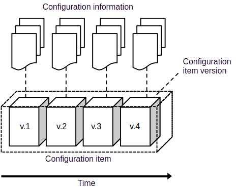
Configuration item as an entity in time.

Configuration item versions are in turn documented in the *configuration information*, a set of documents, models etc, associated with the configuration item (see Figure 1a and Figure 3).

In the most general case, configuration management spans over the following types of configuration items:

As-designed configurations item: (Predicted) characteristics of designed (but not necessarily yet constructed) system element.

As-built configurations items: (Actual and predicted) characteristics of constructed (but not yet put in operation) system element.

As-maintained configuration item: (Actual) characteristics of a system element in operations.

A configuration item should be selected so that it is realized by one system or system element. Configuration items should furthermore be selected so that they can be managed with minimal dependency on other configuration items (modularity). Configuration item selection criteria should therefore consider:

Regulatory requirements
Criticality in terms of risks and safety
Anticipation of new technology replacing old
Interfaces with other configuration items
Procurement
Support and service

Examples:

Components that are procured as a single entity (e.g., an x-ray tube) should be represented by one configuration item that defines the specifications of the component.
System elements that have their own maintenance schedule and maintenance log should be represented by one configuration item that is all the maintenance-related information.
System elements that are developed as one entity, with their own specifications, risk analyses etc. should map to one configuration item.

Configuration: A top-level (root) configuration item; the characteristics of a system element that is managed as an independent entity, often a whole system.

Configuration item version (CIV): A (long exposure time) snapshot of a configuration item between two timestamps, `valid_from` and `valid_to`.

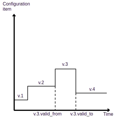
Configuration item as a piecewise constant function of time. A configuration version is a constant segment of the configuration item function. In the figure, v.3 is constant between v.3.valid_from and v.3.valid_to.

If `valid_to` is not set or set to a future date, then the configuration item is currently valid.

For as-designed configuration items valid means released, i.e., formally approved for construction after `valid_from`.

If the last version of an as-designed configuration item has its `valid_to` in the past then it is deleted from the configuration, i.e., the corresponding system element is no longer part of the system.

As built configuration items are kept valid for as long as the system is assumed to be on the market or, in case of medical devices, sometimes indefinitely.

For as-maintained configuration items valid means installed, i.e., operational in a system instance.

An as-maintained configuration item with its `valid_to` in the past is removed from the operational system.

Key configuration item versions (baselines) can also be given a human-readable label, like v2.1.0.

Configuration version: A snapshot of a configuration at a well-defined point in time; a top-level configuration item version.

Configuration baseline: A formally reviewed and approved configuration version that serves as a non-volatile reference point for a well-defined purpose.

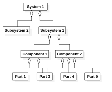
Configuration item graph: A directed acyclic graph (DAG) of configuration items. The graph mirrors the structural decomposition of the system of interest. The reason that the CI graph is not a simple tree is that the same configuration item (e.g., a power outlet) may appear in many branches of the (as-built) configuration item graph in an as-designed configuration. The “acyclic” adjective means that a configuration item can not be part of itself; there can not be any circular part-of associations.

An example of a CI graph is shown in the figure below. Note that Part 3 is part of both Component 1 and Component 2.

Configuration information: A representation of a configuration or a configuration item. Typically a set of documents, source code, models, database records etc that together document the characteristics of a system element (a configuration item).

Information item: A repository of configuration information such as a document, a model, a source code file, or a database record. Information items evolve over time. Their state at a certain point in time is represented by an information item version, a snapshot of the information item at that point in time.

Information item version (IIV): A snapshot of an information item at a well-defined point in time.

Change request: A formal request to change a baseline, e.g., by adding a new function to the system. The change request is not part of the configuration information since it describes a difference between two configuration baselines rather than a configuration baseline.