A segway into information theory

Information theory offers some alternative perspectives on the quantities used in the active inference theory such as surprise, KL divergence, and entropy. I will therefore make a segway into information theory to try to connect some dots.

Information

When an event $E$ with probability $P(E)$ occurs or becomes certain, we gain information about the world.

Desirable properties of a measure of information, $\mathcal I(P(E))$ are:

If $P(E)$ is $1$, then we gain zero information (we already knew what was going to happen).
$\mathcal I(P(E))$ is a continuously increasing function of $\frac{1}{P(E)}$; the smaller the probability, the more information we gain when $E$ happens.
Total information inherent in two (or more) events $E_1$ and $E_2$ should add up so that $\mathcal I(P(E_1), P(E_2)) = \mathcal I(P(E_1)) + \mathcal I(P(E_2))$.

$\mathcal I(P(E))$ is a measure of uncertainty, unexpectedness about events that have not yet occured or surprise about events that have occured.

It can be shown that $\mathcal I(P(E)) = \log_2(\frac{1}{P(E)})$ fulfills the desirable properties (axioms) above. $\mathcal I(P(E))$ is thus a measure of the information we gain when we become certain about the event $E$.

Any logarithm will do but $log_2$ gives the uncertainty in bits which is an intuitive measure for us folks from computer science (the SI unit for information is actually Shannon, Sh but it is often useful to think in bits).

Surprise

Back to active inference and Bayes’ theorem with the notation from the previous post:

$$p(s \mid o) = \frac{p(o \mid s)p(s)}{p(o)}$$

$p(\pmb o)$ is the probability of seeing the observation $o$. The probability $p(o)$ is also in active inference associated with surprise. The smaller the probability, the greater the surprise. Most people would for instance agree that the probability of observing an alien from outer space is small indeed and would therefore be duly suprised should they run into one whereas they would expect to find their car where they parked it and would not be too surprised to find their car in the morning.

The surprise in active inference is measured by the quantity $-\log p(o)$ ¹ which is identical to the definition of information [2]. Surprise in active inference is thus both formally and intuitively the same quantity as information in information theory.

One of the axioms of active inference is that an organism tries to navigate the world so as to remain as unsurprised as possible in relation to its preferred observations². This is equivalent to saying that the organism wants to minimize the information it gets from observations. This information should not be confused with the knowledge that the organism collects all the time to update its internal model so as to minimize future surprises. More on this later.

In the previous post I showed that $\mathcal{F}(o) \geq -\log_2 p(o) = \mathcal I(p(o))$. This means that the variational free energy, $\mathcal{F}(o)$, is an upper bound for the information in the observation $o$. By minimizing $\mathcal{F}(o)$ we minimize the information.

Bayesian surprise

The active inference literature defines another useful kind of surprise which basically indicates how much we change our (prior) beliefs having made an observation if we obey Bayes’ theorem. Bayesian surprise is defined in terms of the dissimilarity between the posterior probability distribution and the prior probability distribution which can be measured with the Kullback-Leibler divergence:

$$D_{KL}\left[p(s \mid o) \mid \mid p(s) \right] := \sum_s \log\left(\frac{p(s \mid o) }{p(s)}\right) p(s \mid o)$$

The difference between surprise and Bayesian surprise can be illustrated with an example: Let’s say that a supporter of a certain former president is certain that the former president is not guilty of any of the crimes he is investigated for. This means that the supporter’s prior belief is $P(\text{not guilty}) = 1.0$.

Let’s say that the investigation finds some rather conclusive evidence of guilt, say a recording of the former president confessing to the crime. The likelihood for a confession given that the former president is not guilty, would in the supporter’s mind be very unlikely, say $P(\texttt{confession} \mid \texttt{not guilty}) = 0.05$. The supporter might put the probability for confession slightly higher in case the former president was guilty, say $P(\texttt{confession} \mid \texttt{guilty}) = 0.1$. Let’s do the math:

$$P(\texttt{not guilty} \mid \texttt{confession}) = $$

$$\frac{P(\texttt{confession} \mid \texttt{not guilty})P(\texttt{not guilty})}{P(\texttt{confession} \mid \texttt{not guilty})P(\texttt{not guilty}) + P(\texttt{confession} \mid \texttt{guilty})P(\texttt{guilty})}$$

What the hard core supporter will believe having heard the evidence (confession) is therefore:

$$P(\texttt{not guilty} \mid \texttt{confession}) = \frac{0.05 * 1.0}{0.05 * 1.0 + 0.1 * 0.0} = 1.0$$

The supporter thus hasn’t changed his or her beliefs at all; the Bayesian surprise is zero.

A trivial but sometimes overlooked conclusion is that if somebody is certain of something then no amount of evidence will move their beliefs. It would be a severe case of Orwellian doublethink to both believe in this ex-president’s absolute innocense and to believe that $P(\texttt{confession} \mid \texttt{not guilty}) = 0.05$. The (fictive) supporters of this particular former president have over the past several years acquired “tremendous” doublethink skills.

While we shouldn’t perhaps be surprised by the erratic behavior of this particular former president, we can quantify the surprise of the supporter associated with a confession mathematically as $\mathcal I(0.05) = -log_2 (0.05) = 4.3$.

Entropy

Continuing down the information theory path, I introduce another quantity called entropy. Entropy is the expected value of information gained from observing outcomes drawn from a certain probability distribution $p(s)$.

$$\mathcal H[p(s)] = \sum_s p(s)log_2(\frac{1}{p(s)})$$

Entropy is a property of a probability distribution. It is always greater than or equal to zero (which probability distribution has the lowest entropy?). $\mathcal H[p(s)]$ is equal to the expected number of bits required to become certain of which event $s$ that has transpired when we know the probability distribution $p(s)$.

Example: Assume that we live in a place where there is a $50\%$ probability of $\texttt{rain}$ and a $50\%$ probability of $\texttt{shine}$.

How big is the entropy, i.e., how many bits do we need to transmit a weather report from this place on average?

$$\mathcal H[p(s)] = \sum_s p(s)log_2(\frac{1}{p(s)}) = 0.5*log_2(\frac{1}{0.5})+0.5*log_2(\frac{1}{0.5}) = 1.0$$

The expected amount of information needed to eliminate the uncertainty is thus exactly one bit; the daily forecast needs to contain one bit of information, zero for rain and one for shine (or vice versa). In other words, when we learn about the weather, we have gained one bit of information.

One bit of information reduces the uncertainty by a factor of two. If we had eight weather types with equal probabilities (more on why this is only valid when the events have equal probabilities below) then we would need three bits of information in the weather report so we could use binary numbers from $\texttt{000}$ to $\texttt{111}$

Encoding and cross-entropy

In the eight-weather example we would quite naturally use three-bit codes (binary numbers) for the weather.

If we would send a stream of such codes, we could decode the stream at the receiving end since we know that each code has exactly three bits.

When we have different probabilities, we want to use shorter than average codes for the common events and longer than average codes for the uncommon events to minimize the average code length.

One such code is the Huffman code. It also satisfied the “prefix rule” stating that no code can be the prefix of any other code. When this is true, a sequence of such codes can be decoded uniquely even though the codes have different lenghts.

Cross-entropy is defined as the average message length in bits of the coding scheme we happen to use to eliminate the uncertainty. There are more or less optimal coding schemes. It can be shown that Huffman code is optimal.

With 8 different types of weather, all with equal probability, we can use three bits to encode the weather as stated before. The cross-entropy is in this case three bits which is also equal to the entropy. Cross-entropy can never be smaller than the entropy. Otherwise we would lose information.

Assume now instead that the probabilities for the eight weather types $\mathbb{s} \in \{\texttt{1}, \texttt{2}, \texttt{3}, \texttt{4}, \texttt{5}, \texttt{6}, \texttt{7}, \texttt{8}\}$ are:

$\mathbb{s}$	$\texttt{1}$	$\texttt{2}$	$\texttt{3}$	$\texttt{4}$	$\texttt{5}$	$\texttt{6}$	$\texttt{7}$	$\texttt{8}$
$P$	$0.25$	$0.25$	$0.125$	$0.125$	$0.0625$	$0.0625$	$0.0625$	$0.0625$

Non-uniform distribution of weather types.

The entropy = average information is in this case $2.75$ bits, i.e. we are wasting bandwidth by assigning three bits to each weather type. We can reduce cross-entropy by assigning likely events shorter codes than unlikely events. We can for instance use this (Huffman) coding:

$\mathbb{s}$	$\texttt{1}$	$\texttt{2}$	$\texttt{3}$	$\texttt{4}$	$\texttt{5}$	$\texttt{6}$	$\texttt{7}$	$\texttt{8}$
$P$	$0.25$	$0.25$	$0.125$	$0.125$	$0.0625$	$0.0625$	$0.0625$	$0.0625$
Code	$\texttt{00}$	$\texttt{01}$	$\texttt{100}$	$\texttt{101}$	$\texttt{1100}$	$\texttt{1101}$	$\texttt{1110}$	$\texttt{1111}$

Weather types encoded by a Huffman code.

The average number of bits sent with this coding scheme turns out to be exactly $2.75$ which is equal to the entropy of the distribution and is therefore optimal.

Kullback-Leibler divergence

I asserted in the previous post that the Kullback-Leibler divergence is a good metric for the dissimilarity between distributions. One way to arrive at this conclusion is by using information theory and encoding. Hang on!

To code the information in an event $s$ with the probability $p(s)$ optimally we need $L_p(s) = \mathcal I(p(s))$ bits (see above), where:

$$L_p(s) = log_2(\frac{1}{p(s)})$$

Let’s say that we assume the distribution to be $q(s)$ instead of $p(s)$ and encode $p(s)$ with an encoding optimal for $q(s)$.

$$L_q(s) = log_2(\frac{1}{q(s)})$$

The cross-entropy (average message length) for the encoding of $p(s)$ can in this case be expressed as a function of two distributions:

$$H[p(s), q(s)] = \sum_s p(s)L_q(s) = \sum_s p(s) log_2(\frac {1}{q(s)})$$

The dissimilarity between the distributions can be measured as the difference between the actual code length (cross-entropy) and the optimal code length (entropy). This difference is called Kullback-Leibler divergence and denoted $D_{KL}[p(s) || q(s)]$.

$$D_{KL}[p(s) || q(s)] = H[p(s), q(s)] – H[p(s)] = $$

$$\sum_s p(s) log_2(\frac {1}{q(s)}) – \sum_s p(s) \log_2\frac{1}{p(s)} = $$

$$\sum_s p(s) log_2(\frac {p(s)}{q(s)})$$

We recognize this expression from the previous post and now we know where it comes from (note though that $p(s)$ and $q(s)$ have traded places compared to the previous post).

Cross-entropy loss in machine learning

As I stated when embarking on this self-taught course on active inference, I wanted to connect some dots between active inference and other areas. Here comes one such connection to machine learning.

A common problem in machine learning is to design and train an algorithm to classify its input into one of a certain number of categories. The first problem that students of machine learning often solve is to classify 28 x 28 pixel images of handwritten numbers into the correct digits, $\texttt{0}$ to $\texttt{9}$. (This is known as the “MNIST problem”.) A simple solution is to build an artificial neural network with 28 x 28 = 784 inputs $o$ and 10 outputs $s \in \{\texttt{0}, \texttt{1}, \texttt{2}, \texttt{3}, \texttt{4}, \texttt{5}, \texttt{6}, \texttt{7}, \texttt{8}, \texttt{9}\}$, one for each digit. The output layer outputs the probabilities $q(s \mid o)$ of the input being each of the ten digits in $\mathbb{s}$ given the input image $o$ (in the vein of active inference framework, I stick with $o$ as the observation, in this case the input pixels).

Artificial neural network for classifying handwritten digits.

The image below illustrates a typical input to the above algorithm and a typical output. The true class of the input is $\texttt{3}$ and the algorithm assigns $\gt 80\%$ probability to it being a $\texttt{3}$. Each of $\texttt{0}$, $\texttt{5}$, and $\texttt{8}$ gets some of the probability mass as the algorithm isn’t entirely certain. We would typically pick the digit with the highest probability when using the algoritm for, say, reading hand-written zip-codes.

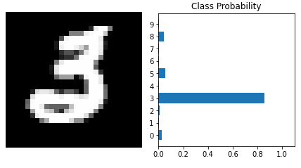
Input and output of the MNIST classifyer.

When training the algorithm above, we would use a large number of images and their corresponding target (ground truth) probability distributions, a training set. An image of $\texttt{3}$ like the one above would in the training set be accompanies by a target distribution $p(\mathbb{s}) = \{\texttt{0}, \texttt{0}, \texttt{0}, \texttt{1}, \texttt{0}, \texttt{0}, \texttt{0}, \texttt{0}, \texttt{0}, \texttt{0}\}$, i.e., with $\texttt{3}$ getting $100\%$ of the probability.

Machine learning uses gradient descent, just like in the active inference. For each input – output pair in the training set of data, the actual output distribution of the algorithm $q(s)$ would be compared with the target distribution $p(s)$ and the dissimilarity, called loss in machine learning, would be used to guide the gradient descent to adjust the algorithm so as to decrease the dissimilarity. The most common dissimilarity metric in a machine learning classification scenario is, like in active inference, the Leibler-Kullback divergence which we derived above using the cross-entropy concept. The corresponding loss function in machine learning is therefore called cross-entropy loss which is a rather obscure term if one doesn’t know the background.

Besides that we now know where the term cross-entropy loss comes from, it is interesting to note that training of a classifier in machine learning uses the same type of method (gradient descent) and loss function (cross-entropy loss) that may be used in active inference. The difference is that in machine learning the method and loss is used for training the algorithm, i.e., learning the model of the world, whereas in active inference they are used for inference, i.e., for predicting the state of the world, given an existing model of the world. (Gradient descent may also be used by the brain for updating its model of the world but that is a different story.)

Summary

As I wrote in the beginning of this post, I’m not at this point sure exactly how information theory can inform (as it were) active inference but as both deal with the same concepts, it seems likely that there are some intersting connections. Just like there are connections between active inference and machine learning and (perhaps) active inference and consciousness.

Links

[1] Olivier Rioul. This is IT: A Primer on Shannon’s Entropy and Information.
[2] Thomas Parr, Giovanni Pezzulo, Karl J. Friston. Active Inference.
[3] Ryan Smith, Karl J. Friston, Christopher J. Whyte. A step-by-step tutorial on active inference and its application to empirical data. Journal of Mathematical Psychology. Volume 107. 2022.

$\log$ can be interpreted as any logarithm here and going forward. In information theory a 2-logarithm is usually convenient. In most of the AIF literature the natural logarithm is used. ↩︎
The AIF literature is ambiquous regarding how preferences are actually encoded. There are passages that seem to indicate that the prior beliefs $p(s)$ hold not only expectations but also preferences; what is expected is sometimes also preferred whereas other passages claim that the priors do not encode any preference but just pure expectations. I will try to sort this out in later posts. ↩︎

\(\mathbb{s}\)	\(\texttt{1}\)	\(\texttt{2}\)	\(\texttt{3}\)	\(\texttt{4}\)	\(\texttt{5}\)	\(\texttt{6}\)	\(\texttt{7}\)	\(\texttt{8}\)
\(P\)	\(0.25\)	\(0.25\)	\(0.125\)	\(0.125\)	\(0.0625\)	\(0.0625\)	\(0.0625\)	\(0.0625\)

\(\mathbb{s}\)	\(\texttt{1}\)	\(\texttt{2}\)	\(\texttt{3}\)	\(\texttt{4}\)	\(\texttt{5}\)	\(\texttt{6}\)	\(\texttt{7}\)	\(\texttt{8}\)
\(P\)	\(0.25\)	\(0.25\)	\(0.125\)	\(0.125\)	\(0.0625\)	\(0.0625\)	\(0.0625\)	\(0.0625\)
Code	\(\texttt{00}\)	\(\texttt{01}\)	\(\texttt{100}\)	\(\texttt{101}\)	\(\texttt{1100}\)	\(\texttt{1101}\)	\(\texttt{1110}\)	\(\texttt{1111}\)