In this post we will take a deeper look at how, according to the active inference framework (AIF), an agent infers controller states (internal states) representing system states (external states) based on observations. We call this process perceptual inference.
The simple example in the previous post showed how the human brain could according to AIF turn an observation into a probability over controller states representing what it observes using its generative model and Bayes’ theorem. Since there were only two interesting system states in the garden scenario, a frog and a lizard, it was possible to calculate the posteriori probability distribution for the controller state as a closed-form expression (a “frog” with 73% probability). In real life there are too many possible controller states for the brain to be able to calculate the probability distribution of controller states analytically.
This post describes how, according to active inference framework (AIF), an agent gets around the messy intractability of reality.
We don’t really know what’s out there
AIF posits that the generative model translates observations to probabilities for controller states that are representations of system states. The generative model can be compared to a map. The cities on the map represent cities in the real world. When using the map, we shift our attention to the next city on the map when we physically arrive there. We shall in future posts see how the generative model can be used to infer actions that can take the organism from the current state to a future state analogous to how we can use the map to infer how to drive from the current city to the next city. In both cases we need to know where we are now. The ultimate purpose of perceptual inference is not to give us a high-definition internal image of what we see but to infer in which controller state we are so that we can decide what to do next to stay alive and do what we want.
Evolution has given us generative models that are useful. They allow us to create useful internal representations (controller states) of the state of the world (system states) and to infer actions to get from one state to the next. If this would not be the case, we would not be here. The usefulness of the generative model is taken as an axiom in the theory of active inference.
A maybe trivial, but sometimes forgotten, fact is that a model is not the reality; the map is not the terrain; the controller state is not the system state. An agent can only create, use, and store useful representations of the world in the form of controller states. These representations only capture certain vital aspects of the system states. Ontologically the model and the real world are two very different animals.
In case of frogs and lizards there is a straightforward correspondence between the controller state and the animal out there in the wild.
Some, perhaps all, controller states are also associated with an attribute that has not so far been observed in the real world, namely subjective experience. Examples of subjective experiences are green and pain [5]. We see not only a frog but a green frog. We not only see that our tooth is cracked and feel the crack with our tongue, we also feel the pain and can tell where the tooth is located in our body.
Controller states associated with subjective experiences are arguably useful as they are easy to remember, communicate, and act on. In some cases, like in case of severe pain, they are imperative to act on thereby giving a very strong motivation for the agent to stay alive (and, under the influence of other subjective experiences, procreate). I will return to this topic in a future post.
Some notation and ontology
We will in this post, like in the previous post, assume that all distributions are categorical, i.e., their supports are vectors of discrete events:
$$p(o) = \text{Cat}(o, \pmb{\omega)}$$
$$p(s) = \text{Cat}(s, \pmb{\sigma)}$$
Again, the above distributions mean for instance that \(p(o_i) = P(O = o_i) = \omega_i\), i.e., \(\pmb{\omega}\) is a vector of probabilities.
As stated before, the optimal way, according to AIF, for an agent to arrive at the probabilities for controller states is by using Bayes’ theorem:
$$p(s \mid o) = \frac{p(o, s)}{p(o)} = \frac{p(o \mid s)p(s)}{p(o)} = \frac{p(o \mid s)p(s)}{\sum_s p(o \mid s)p(s)}$$
\(p(o, s)\) is the brains generative model (we will later add action to the model). It models how observations and controller states are related in general. It packs all information needed for perceptual inference.
\(p(o, s) = p(o \mid s)p(s)\) where:
- \(p(s)\) is the agent’s expectations, “priors”, about the probabilities of each possible controller state in the vector of all potential controller states \(\pmb{S}\) prior to an observation.
- \(p(o \mid s)\), the likelihood, is the probability distribution of observations given a certain controller state \(s\).
The last piece of Bayes’ theorem is the evidence \(p(o)\). It is simply the overall probability of a certain observation \(o\). It would ideally need to be calculated using the law of total probability by summing up the contributions to \(p(o)\) from all possible controller states:
$$p(o) = \sum_{s} p(o \mid s)p(s)$$
Since there is a large number of controller states (corresponding to an even larger number of system states), this sum would be very long making the evidence intractable.
Some intuition
The prior \(p(s)\) is according to Bayes’ theorem modulated by the ratio \(\frac{p(o \mid s)}{p(o)}\) to get the posterior probabilities of controller states. Let’s look at two examples to gain some intuition about this ratio.
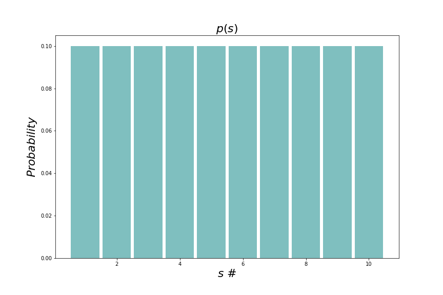
Let’s say that we are looking at animals in a zoo and want to identify the species by doing an observation. We know that there are exactly ten animals, all of different species, in this small zoo and that the priori probability for seeing a certain species is the same for all ten animals (here identified with numbers from one to ten). \(p(s)\) is therefore a uniform distribution that looks like this:
In the first case we assume that our observation is whether the sun is shining or not. We know that where we are, the sun shines \(50\%\) of the time meaning that we get the following conditional probability in the numerator
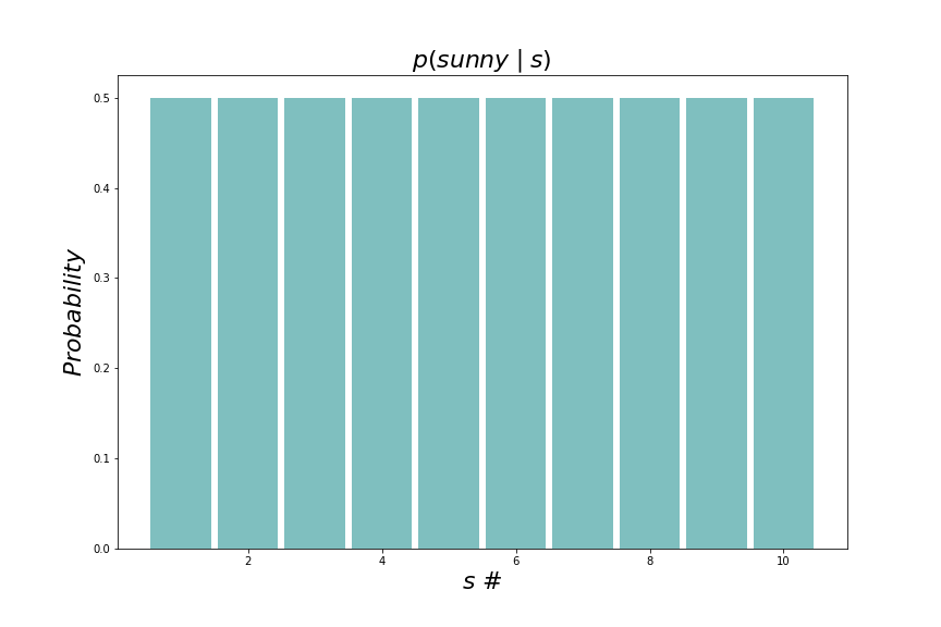
As stated above as an assumption, the evidence (denominator) is \(p( \texttt{sunny}) = 0.5\). Therefore the ratio \(\frac{p(\texttt{sunny} \mid s)}{p(\texttt{sunny})} = 1.0\) for all beliefs meaning that the posterior is equal to the prior; we have not learned anything from the observation which we of course new in forehand since knowing the weather doesn’t tell us very much about the animals in the zoo.
In the second case we are smarter and try to find a feature to observe that actually says something about the animal we are looking at. Let’s say that one of the animals is a dromedary and we observe a hump. Only the dromedary sports a hump so we are certain to observe hump for the \(\texttt{dromedary}\) controller state and certain not to observe a hump for any other controller state. The numerator of the ratio now looks like this:
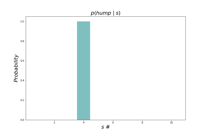
#4 is the \(\texttt{dromedary}\) controller state.
The total probability of observing a hump is now \(0.1\) since only one of the ten animals has a hump. The ratio \(\frac{p(\texttt{hump} \mid s)}{p(\texttt{hump})} = 10\) for the \(\texttt{dromedary}\) controller state (\(s\)). This means that if we observe a hump, the probability of a \(\texttt{dromedary}\) controller state should increase by a factor of \(10\). With the uniform prior probability distribution, the posterior probability for a \(\texttt{dromedary}\) now becomes \(10 \times 0.1 = 1.0\). We have gained enough information to now be certain that our controller state is \(\texttt{dromedary}\).
How to calculate the intractable
There are ways to find approximations \(q(s)\) to the optimal posterior distribution over controller states given an observation \(p(s \mid o)\) without having to calculate \(p(o)\):
$$q(s) \approx p(s \mid o) = \frac{p(o \mid s)p(s)}{p(o)}$$
Although \(q(s)\) depends on \(o\) indirectly, this dependency is usually omitted in AIF notation. \(q(s)\) can be seen as just a probability distribution that is an approximation of another probability distribution that in turn depends on \(o\).
The canonical method to find the approximate probability distribution over controller states \(q(s)\) is variational inference which can be formulated as an optimization problem. There is some empirical evidence suggesting that the brain actually does something similar [6].
\(q(s)\) is usually assumed to belong to some tractable distribution like a multidimensional Gaussian. Variational inference finds the optimal parameters of the distribution, in the Gaussian case the covariance matrix) and the mean vector. In the following the set of parameters is denoted \(\theta\).
There are several optimization methods that can be used for finding the \(\theta\) that minimizes the dissimilarity between \(q(s \mid \theta)\) and \(p(s \mid o)\). A popular one is gradient descent that is also used in machine learning. We here assume that the inference of \(q(s \mid \theta)\) is fast enough for \(o\) and the generative model to remain constant during the inference.
Optimization minimizes a loss function \(\mathcal L(o, \theta)\). The Kullback-Leibler divergence 1 \(D_{KL}\) measures the dissimilarity between two probability distributions and is thus a good loss function candidate for active inference:
$$\mathcal L(o, \theta) = D_{KL}\left[q(s \mid \theta) \parallel p(s \mid o) \right] := \mathbb E_{q(s \mid \theta)}[\ln q(s \mid \theta) – \ln p(s \mid o)] $$.
\(\mathcal L(o, \theta)\) equals zero when both distributions are identical. It can be shown that \(\mathcal L(o, \theta) \gt 0\) for all other combinations of distributions.
The loss function unpacked
Let’s try to unpack \(\mathcal L(\theta, o)\) into something that is useful for gradient descent:
$$\mathcal L(o, \theta) = D_{KL}\left[q(s \mid \theta) \parallel p(s \mid o) \right] = \mathbb E_{q(s \mid \theta)}[\ln q(s \mid \theta) – \ln p(s \mid o)] =$$
$$\mathbb E_{q(s \mid \theta)}[\ln q(s \mid \theta) + \ln p(o) – \ln p(o \mid s) – \ln p(s)] = $$
$$\mathbb E_{q(s \mid \theta)}[\ln q(s \mid \theta) – \ln p(o \mid s) – \ln p(s)] + \ln p(o) = $$
$$\mathbb E_{q(s \mid \theta)}[\ln q(s \mid \theta) – \ln p(o, s)] + \ln p(o) = $$
$$\mathcal{F}(o, \theta) + \ln p(o)$$
With:
$$\mathcal{F}(o, \theta) = \mathbb E_{q(s \mid \theta)}[\ln q(s \mid \theta) – \ln p(o, s)] $$
\(\mathcal{F}(o, \theta)\) is called variational free energy or just free energy 2. Since \(\ln p(o) \) doesn’t depend on \(\theta\), \(D_{KL}\left[q(s \mid \theta) \parallel p(s \mid o) \right]\) is minimized when \(\mathcal{F}(o, \theta)\) is minimized meaning that we can replace our earlier loss function with free energy.
Given well-behaved distributions, \(\mathcal{F}(o, \theta)\) can be made differentiable with respect to \(\theta\) which means that it can be minimized using gradient descent. An estimate of the loss function in each iteration can be found using Monte Carlo integration which means that we only take a few samples from \(q(s \mid \theta)\), not the full distribution, do the multiplications and the summation. We then calculate the gradient of this sum with respect to \(\theta\) and adjust \(\theta\) with a small fraction (the learning rate) of the negative gradient [1]. Note that \(p(s)\) and \(p(o \mid s)\) are assumed to be quantities available to the agent for use in the calculation of the loss function.
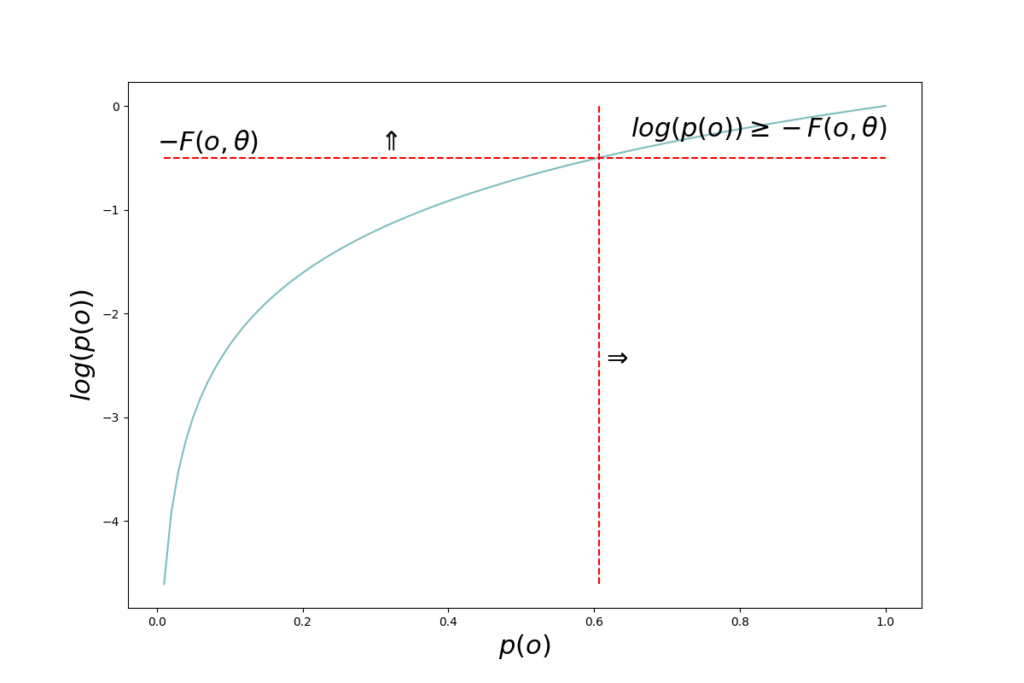
The quantity \(– \mathcal{F}(o, \theta)\) is in Bayesian variational methods denoted evidence lower bound, ELBO, since \(D_{KL}\left[q(s \mid \theta) \parallel p(s \mid o)\right] \geq 0\) and therefore \(\ln p(o) \geq – \mathcal{F}(o, \theta)\).
The quantity \(– \ln p(o) \) remains unchanged during perceptual inference. The observation is what it is as long as the agent doesn’t change something in its environment that would cause the observation to change as a consequence.
Surprise
The quantity \(– \ln p(o)\) can be seen as the “residual” of the variational inference process. It is the part that can not be optimized away, regardless of how accurate a variational distribution \(q(s \mid \theta)\) we manage to come up with. \(p(o)\) is the probability of the observation. If the observation has a high probability, it was “expected” by the model. Low probability observations are unexpected. \(– \ln p(o) \) is therefore also called surprise. High probability \(p(o)\) means low surprise and vice versa.
From above we have \(\ln p(o) \geq – \mathcal{F}(o, \theta) \Rightarrow -\ln p(o) \leq \mathcal{F}(o, \theta)\) meaning that the free energy is an upper bound on surprise; surprise is always lower than or equal to free energy.
According to AIF, a biological agent strives to minimize surprise at all times as a large surprise means that the system is in a non-viable state. To minimize surprise, the agent not only infers a controller state but also takes action to perturb the system, thereby lowering surprise. Minimizing surprise will be the topic of coming posts.
Links
[1] Khan Academy. Gradient descent.
[2] Volodymyr Kuleshov, Stefano Ermon. Variational inference. Class notes from Stanford course CS288.
[3] Thomas Parr, Giovanni Pezzulo, Karl J. Friston. Active Inference.
[4] Hohwy, J., Friston, K. J., & Stephan, K. E. (2013). The free-energy principle: A unified brain theory? Trends in Cognitive Sciences, 17(10), 417-425.
[5] Anil Seth. Being You.
[6] Andre M. Bastos, W. Martin Usrey, Rick A. Adams, George R. Mangun, Pascal Fries, Karl J. Friston,
Canonical Microcircuits for Predictive Coding, Neuron, Volume 76, Issue 4, 2012, Pages 695-711.
- Technically \(D_{KL}\) is a functional which is a function of one or more other functions. \(D_{KL}\) is a function of \(q(s, \pmb \theta)\). The square brackets around the argument are meant to indicate a functional. Intuitively one can think of a functional as a function of a large (up to infinite) number of parameters, namely all the values of the functions that are its arguments. ↩︎
- The term is borrowed from thermodynamics where similar equations arise. Knowing about thermodynamics is not important for understanding AIF though. \(\mathcal{F}(o, \theta)\) is sometimes written as a functional like this: \(\mathcal{F}[q; o]\). This is a more general expression as it doesn’t make any assumptions about the probability distribution \(q\). ↩︎