Assume that surprise is defined as \(-\log p(o)\) [1, p.18]. I will in this post try to illustrate why this is a good measure of surprise
$$p(o) = \sum_i p(o \mid s_i)p(s_i)$$
where \(p(s_i)\) yields the probability of each currently possible state of the world and \(p(o \mid s_i)\) yields the probability of observation \(o\), when the state is \(s_i\). In this post we assume that only one \(p(s_i) = p(s_{expected})\) is non-zero at each point in time. It’s either best to go left or to go right but never both.
To understand why surprise is a useful quantity, we use an example. Assume that we are observing an object that can be either a circle, a hexagon or a diamond. These are the three states of the world within our very limited scope. The real-world states are are represented by mental states denoted \(s_c\), \(s_h\), and \(s_d\) respectively. (Sorry for yet another unimaginative example. I hope it conveys the idea despite its dullness.) The state space in this example is discrete meaning that the states are enumerable.
The observation gleaned from somewhere in the visual cortex is that of “shape”. There are three possible shapes in our limited observation repertoire: circular, hexagonal, and diamond-like. Note that while the shapes linguistically map one-to-one onto the objects, there is a clear ontological distinction between observations and (mental) states.

The association between observations and states is described by the joint probability distribution \(p(o, s)\) illustrated in the figure below.
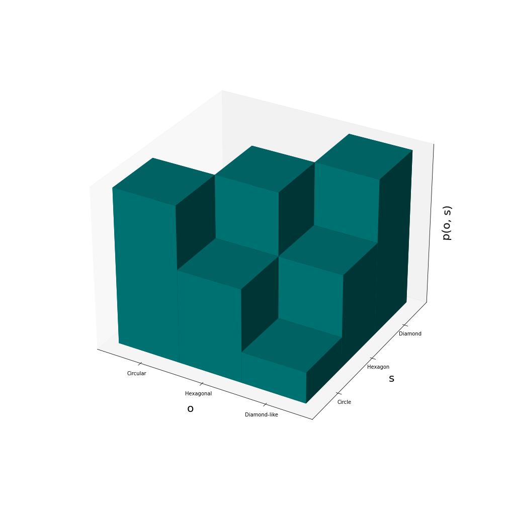
From the figure we can conclude that the observation of a diamond-shape has high probability when the mental state is a diamond whereas the observatoin of a diamond-like shape is improbable when the mental state is a circle. It is somewhat probable to observe a circular shape when the state is a hexagon (e.g., when the observation is made from afar or in fog).
We will now compare the surprise in two different scenarios.
In the first scenario the expected state of the world is a hexagon (don’t ask why) in this simple example meaning that \(p(s_h) = 1.0\)1 while \(p(s_c) = p(s_d) = 0\). In this scenario the actor observes a hexagonal shape. \(p(o) = \sum_i p(o \mid s_i)p(s_i) = p(o \mid s_h)p(s_h)\). \(p(o \mid s_h)\) is illustrated in the figure below.
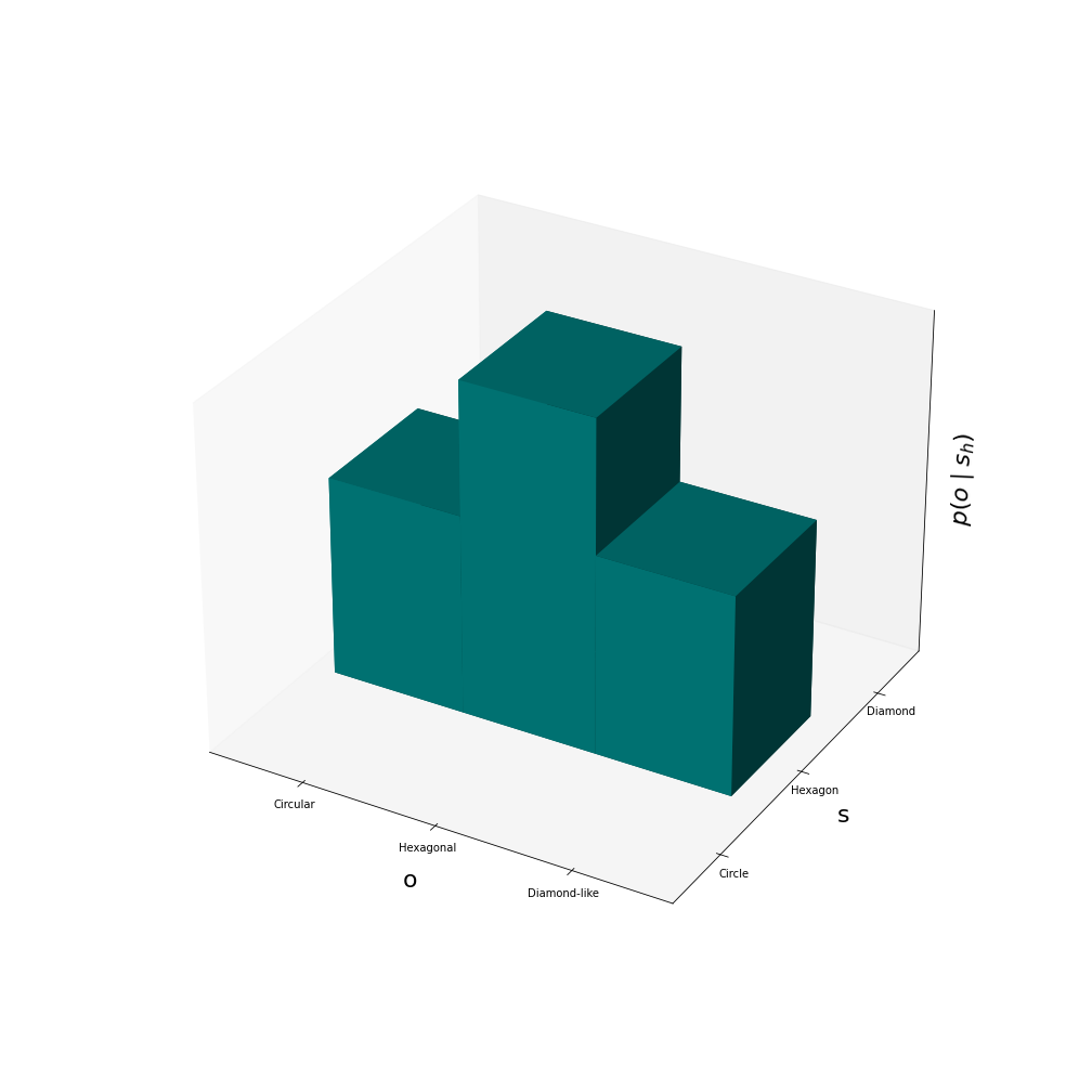
Conditional probability distribution \(p(o \mid s_h)\).
In this first scenario \(p(o_h \mid s_h) \approx 0.45\) (note that the probabilities summed over observations add up to one since this is the total probability distribution). The surprise is thus \(-log(1.0 \times 0.45) \approx 0.8\).
In the other scenario the expected state is instead a circle but the actor observes a diamond-like shape. The conditional probability distribution looks like this:
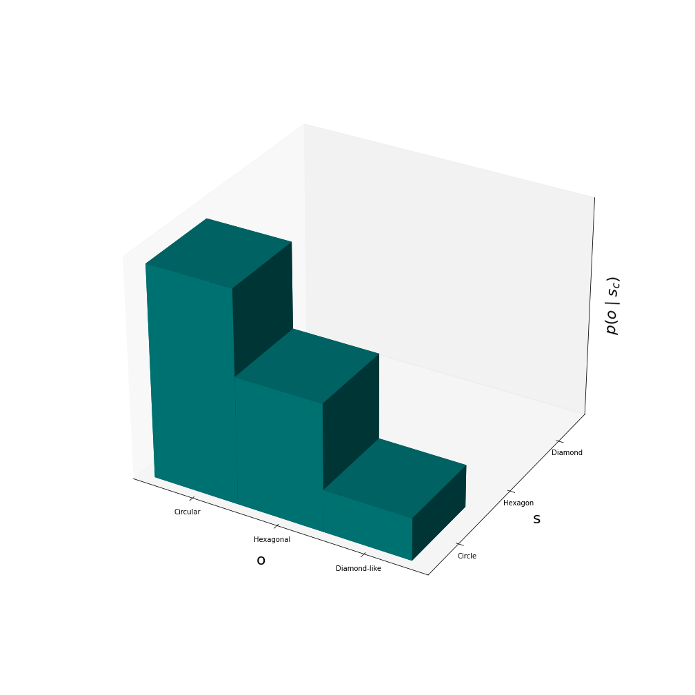
It is rather improbable to observe a diamond-like shape when the expected state is a circle. In this second scenario \(p(o_d \mid s_c) \approx 0.11\) and the surprise is \(-log(1.0 \times 0.11) \approx 2.19\) which is significantly higher than the surprise in the first scenario.
The actor is intuitively and mathematically more surprised i the second scenario where the observation isn’t very likely for the expected prior. In general, for the surprise to be low, the observation must be probable for the expected state. The probability for the observation given a certain state is given by the brains generative model and quantified by \(p(o \mid s)\). If we assume that there is only one expected state as in the example above, then the surprise collapses to \(-log (p(o \mid s_{expected})p(s_{expected}))\).
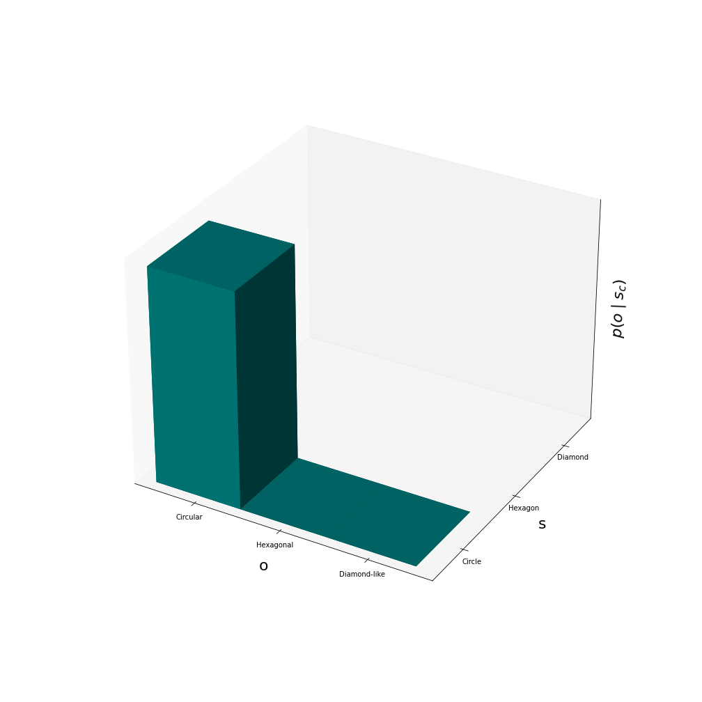
Worth noting is also that the more specific the generative model is, the smaller the surprise. The most specific model is the one where \(p(o \mid s_{expected})p(s_{expected}) = 1.0\). This is illustrated in the figure below. The least specific model is instead one that assigns equal probabilities for seeing all shapes regardless of the true state.
Links
[1] Thomas Parr, Giovanni Pezzulo, Karl J. Friston. Active Inference.
[2] Ryan Smith, Karl J. Friston, Christopher J. Whyte. A step-by-step tutorial on active inference and its application to empirical data. Journal of Mathematical Psychology. Volume 107. 2022.
[3] Beren Millidge, Alexander Tschantz, Christopher L. Buckley. Whence the Expected Free Energy. Neural Computation 33, 447–482 (2021).
- In reality it is never a good idea to have a prior that equals 1.0 because that would mean that no observation would sway your belief. Unfortunately we see a lot of such 1.0 priors in the world today, especially in politics and religion. ↩︎